RNA-seq Tutorial- HISAT2, StringTie and Ballgown*
Now users can run Rstudio as app in CyVerse Discovery Environment. Please see this updated wiki page to run New RNA-Seq Tuxedo protocol - RNA-seq Tutorial- HISAT2, StringTie and Ballgown using DE and Rstudio-Ballgown*
New RNA-Seq tuxedo protocol using the Discovery Environment
Rational and background
RNA-seq involves preparing the mRNA which is converted to cDNA and provided as input to next generation sequencing library preparation method. Prior to RNA-seq there were hybridization based microarrays used for gene expression studies, the main drawback was the poor quantification of lowly and highly expressed genes. RNA-seq provides distinct advantages over microarrays, it provides better insights into alternative gene splicing, post-transcriptional modifications, gene fusion and deferentially expressed genes and thus helping to understanding the gene structure and expression patterns of genes across different samples, treatment conditions and time points. The ease of sequencing and the low cost have made RNA-seq a workhorse in transcriptomic studies and viable option even for small scale labs. But the main challenge remains in analyzing the sequenced data.
The current ecosystems of RNA-seq tools provide a varied ways of analyzing RNA-seq data. Depending on the experiment goal one could align the reads to reference genome or pseduoalign to transcriptome and perform quantification and differential expression of genes or if you want to annotate your reference, assemble RNA-seq reads using a denvo transcriptome assembler. Here we focus on workflows that align reads to reference genomes. The most commonly cited and widely used workflow is the Tuxedo protocol (Tophat,Cufflinks,Cuffdiff)developed by Cole Trapnell et al. The main drawback of this workflow is the ability to scale i.e they tend to take more runtime compared to newly updated Tuxedo protocol(HISAT,StringTie,Ballgown) by Mihaela Pertea et al. This updated Tuxedo protocol not only scales but is more accurate in detecting deferentially expressed genes.
In this example we will compare gene transcript abundance drought sensitive sorghum line under drought stress(DS) and well-watered (WW) condition. The expression of drought-related genes was more abundant in the drought sensitive genotype under DS condition compared to WW.
We will use RNAseq to compare expression levels for genes between DS and WW- samples for drought sensitive genotype IS20351 and to identify new transcripts or isoforms. In this tutorial, we will use data stored at the NCBI Sequence Read Archive.
- Align the data to the Sorghum v1 reference genome using HISAT2
- Transcript assembly using StringTie
- Identify differential-expressed genes using Ballgown
- Use Atmosphere to visually explore the differential gene expression results.
If you do not have an account, please see one of the on-site CyVerse staff for a temporary account.
Here is the webinar that explains more about the new pipeline:
Specific Objectives
By the end of this module, you should
- Be more familiar with the DE user interface
- Understand the starting data for RNA-seq analysis
- Be able to align short sequence reads with a reference genome in the DE
- Be able to analyze differential gene expression in the DE and Atmosphere
Note on Staged Data:
Several of the methods in this tutorial can take 2 to 4 hrs to complete on a full-sized data set. So that you can complete the tutorial in the allotted time, we have pre-staged input and output files in the 'Community Data' folder for each step. You can start your analyses then skip to the next step using pre-staged data.
Original data from NCBI Sequence Read Archive study re accessible through GEO Series accession number GSE80699
- GSM2133750 IS20351_WW_1
- GSM2133751 IS20351_WW_2
- GSM2133752 IS20351_WW_3
- GSM2133753 IS20351_DS_1
- GSM2133754 IS20351_DS_2
- GSM2133755 IS20351_DS_3
Paper Reference for dataset: Drought stress tolerance strategies revealed by RNA-Seq in two sorghum genotypes with contrasting WUE,
Alessandra Fracasso, Luisa M. Trindade and Stefano Amaducci; DOI: 10.1186/s12870-016-0800-x, May 2016
The Staged Fastq Data can be found in the
Community Data -> iplantcollaborative -> example_data -> HISAT2_StringTie_Ballgown -> reads

Section 1: Align reads to reference using HISAT2 aligner
Hisat2 is another efficient splice aligner which is a replacement for Tophat in the new Tuxedo protocol. Like Tophat2 it uses one global FM index along with several small local FM indexes to build an efficient data structure which helps speed its alignment several times faster than Tophat2.
HISAT2 paper: HISAT: a fast spliced aligner with low memory requirements
Reference Manual
a) Open HISAT2 app
Click on Operation -> Categories -> Mapping -> HISAT2-index-align.

b) Click on the name of the App to open it.

c) In the Input section,you need to first select the a reference genome and annotation file either from the drop list or upload a fasta for the genomes or gtf annotation file.
Here we upload the reference genome file from:
Reference genome : Community Data ->iplantcollaborative->example_data->HISAT2_StringTie_Ballgown->Sorghum_bicolor.Sorbi1.20.dna.toplevel.fa

you can click 'Add' at the top right of the FASTQ File(s) box to navigate to the folder containing the FASTQ files: For paired end data add the read 1 gzipped files for all samples then followed by read 2 files in gzipped format.
Select File type as PE since we are using paired end data set.

Note: For multiple input files, it is convenient to open a separate data window, navigate to the above folder and drag all of files into the input data box. Each of the input files will be processed independently. For convenience, a batch of FASTQ files can be analyzed together but these files can also be processed concurrently in independent STAR runs
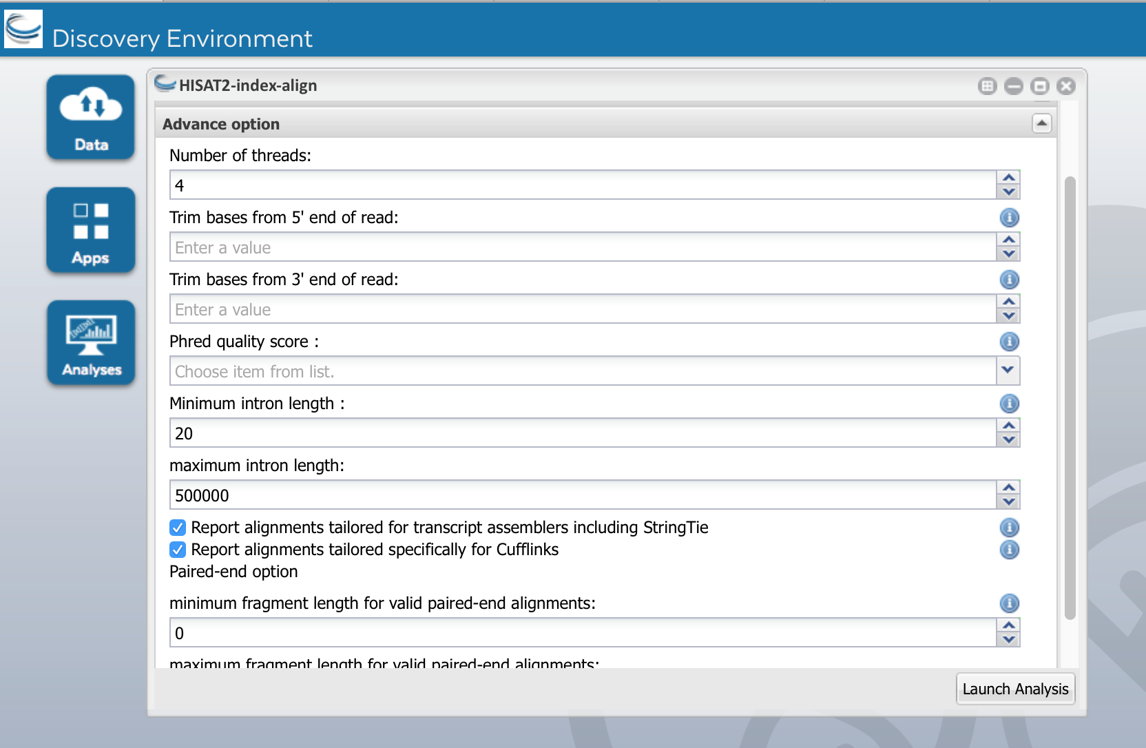
Under advance options select to make alignments compatible with StringTie and Cufflinks for downstream analysis
d) Start the analysis by clicking the Launch Analysis button, naming the analysis 'HISAT2' in the dialog box. Reasonable default options are provided for the analysis settings.

e) HISAT2 will require some time to complete its work on each sample. Click on the Analyses icon to view the status of your submitted analysis.

f) When the analysis is complete, navigate to the results under your 'analyses' folder. The principle outputs from HISAT2 are BAM files, each set of alignments in a bam_output folder, bam file corresponding to the name of the original Fastq file. This is the most time-consuming step of this training module. If your analysis has not completed in time, you can skip ahead by using the pre-computed results:
Community Data ->iplantcollaborative->example_data->HISAT2_StringTie_Ballgown-> HISAT2_results
In the HISAT2_results folder, you should see these folders:
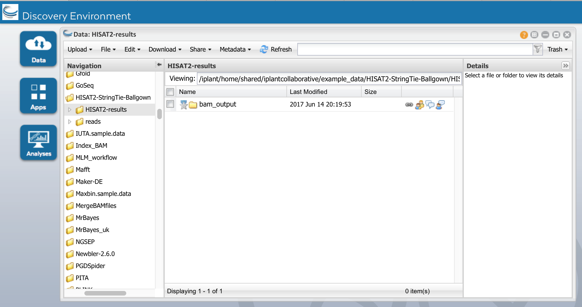
HISAT2_results: The result directory for the HISAT2 runs contain the following
bam_output: directory of alignment files coordinate sorted in bam format for each sample, along with their index bai files
We will use the bam_output folder to assemble transcripts using Stringtie.
Section 2: Assemble transcripts with StringTie-1.3.3
StringTie like Cufflinks2 assembles transcripts from RNA seq reads aligned to the reference and does quantification. It follows a netflow algorithm where it assembles and quantitates simultaneously the highly expressed transcripts and removes reads associated with that transcripts and repeats the process until all the reads are used. This algorithm improves the run time for StringTie using less memory compared to Cufflinks2. If provided with a reference annotation file Stringtie uses it to construct assembly for low abundance genes, but this is optional. Alternatively, you can skip the assembly of novel genes and transcripts, and use StringTie simply to quantify all the transcripts provided in an annotation file
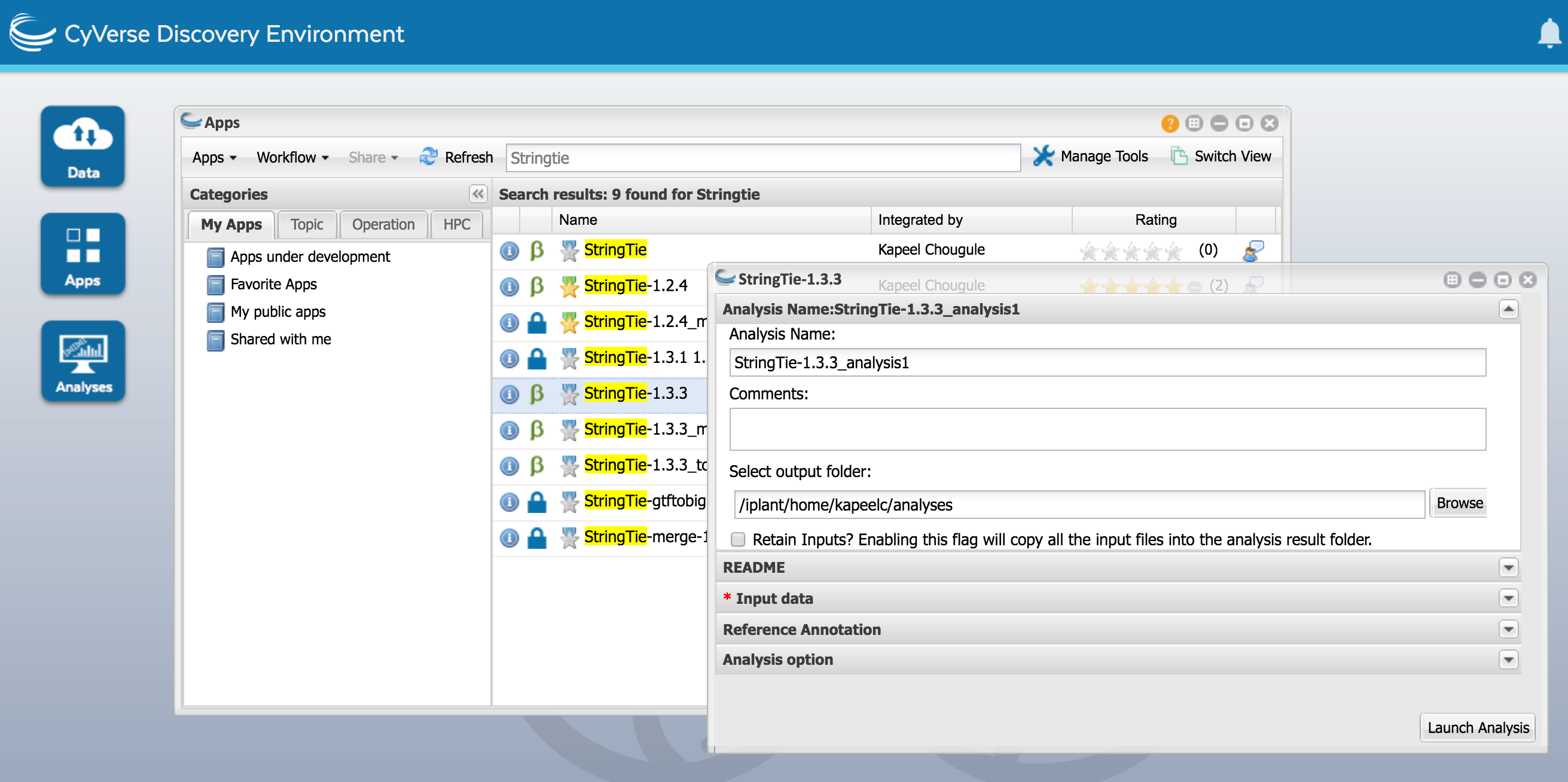
a) Click on the Apps icon and find StringTie-1.3.3. Open it. Name the analysis as StringTie-1.3.3
b) In the 'Select Input data' section, add the 'bam' files by navigating to the bam_output folder from HISAT2 (above) and select and drag all bam files into the input box. For convenience, a batch of HISAT2 bam files can be analyzed together but these files can also be processed concurrently in independent StringTie runs. The path for the HISAT2 bam files
Community Data ->iplantcollaborative->example_data->HISAT2_StringTie_Ballgown-> bam_output

c) In the Reference Annotaiton section, select reference annotation Sorghum_bicolor.Sorbi1.20.gtf.

d) Run StringTie-1.3.3. When it is complete, you will see the following outputs
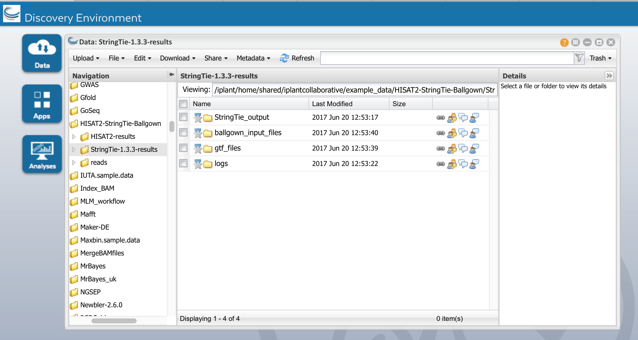
StringTie_output contains the following files:
- Stringtie's main output is a GTF file containing the assembled transcripts e.g:IS20351_DS_1_1.gtf
- Gene abundances in tab-delimited format e.g IS20351_DS_1_1_abund.tab
- Fully covered transcripts that match the reference annotation, in GTF format e.g IS20351_DS_1_1.refs.gtf
Examine the GTF file, IS20351_DS_1_1.gtf This file contains annotated transcripts assembled by StringTie-1.3.3, using the annotated transcripts selected from the reference file uploaded in the StringTie-1.3.3 app as a guide.This file gives normalized expression metrics in both FPKM and TPM along with per base coverage
# stringtie IS20351_DS_1_1.sorted.bam -o IS20351_DS_1_1.gtf -G Sorghum_bicolor.Sorbi1.20.gtf -p 4 -m 200 -c 2.5 -g 50 -f 0.1 -C IS20351_DS_1_1.refs.gtf -A IS20351_DS_1_1.abund.tab
# StringTie version 1.3.3
8       StringTie       transcript      10354   14469   1000    +       .       gene_id "STRG.1"; transcript_id "STRG.1.1"; cov "3.489598"; FPKM "0.801415"; TPM "0.990349";
8       StringTie       exon    10354   10640   1000    +       .       gene_id "STRG.1"; transcript_id "STRG.1.1"; exon_number "1"; cov "1.000000";
8       StringTie       exon    13241   13900   1000    +       .       gene_id "STRG.1"; transcript_id "STRG.1.1"; exon_number "2"; cov "5.615151";
8       StringTie       exon    13975   14469   1000    +       .       gene_id "STRG.1"; transcript_id "STRG.1.1"; exon_number "3"; cov "2.098990";
8       StringTie       transcript      43183   43920   1000    +       .       gene_id "STRG.2"; transcript_id "STRG.2.1"; cov "2.972900"; FPKM "0.682751"; TPM "0.843710";
8       StringTie       exon    43183   43920   1000    +       .       gene_id "STRG.2"; transcript_id "STRG.2.1"; exon_number "1"; cov "2.972900";
8       StringTie       transcript      43997   44781   1000    +       .       gene_id "STRG.3"; transcript_id "STRG.3.1"; cov "6.772846"; FPKM "1.555440"; TPM "1.922136";
8       StringTie       exon    43997   44216   1000    +       .       gene_id "STRG.3"; transcript_id "STRG.3.1"; exon_number "1"; cov "9.109091";
Section 3: Merge all StringTie-1.3.3 transcripts into a single transcriptome annotation file using StringTie-1.3.3_merge
StringTie-merge like Cufflinks-merge uses the same principle of merging the transcript assemblies from samples into a consolidated annotation set. This merging steps helps restore full length of the structure transcript especially for transcript assembled with low coverage.The main purpose of this application is to make it easier to make an assembly GTF file suitable for use with Ballgown. A merged, empirical annotation file will be more accurate than using the standard reference annotation, as the expression of rare or novel genes and alternative splicing isoforms seen in this experiment will be better reflected in the empirical transcriptome assemblies.
a) Open the StringTie-1.3.3_merge app. Under 'Input Data', browse to the results of the StringTie-1.3.3 analyses (gtf_out). Select the all GTF files as input for StringTie-1.3.3_merge.

b) Under Reference Annotation, select the Sorghum_bicolor.Sorbi1.20.gtf.

c) Run the App. When it is complete, you should see the following outputs under StringTie-1.3.3_merge_results:

We will use the merged.out.gtf with StrignTie-1.3.3 app again
Section 4: Create Ballgown input files using with StringTie-1.3.3
We will use StringTie-1.3.3 again to assemble transcripts but this time will will use the consolidated annotation file we got from StringTie-1.3.3_merge step. This will re-estimate the transcript abundances using the merged structures but reads may need to be re-allocated for transcripts whose structures were altered by the merging step. We will set the option -B, e of StringTie. These options are set by checking the two boxes at the bottom of the 'analysis option' section of the app. This will create table count files (*ctab files) for each sample to be used in Ballgown for differential expression. Name the analysis "StringTie-1.3.3_from_merged_annotation"

Run the App. When it is complete, you should see the following outputs under
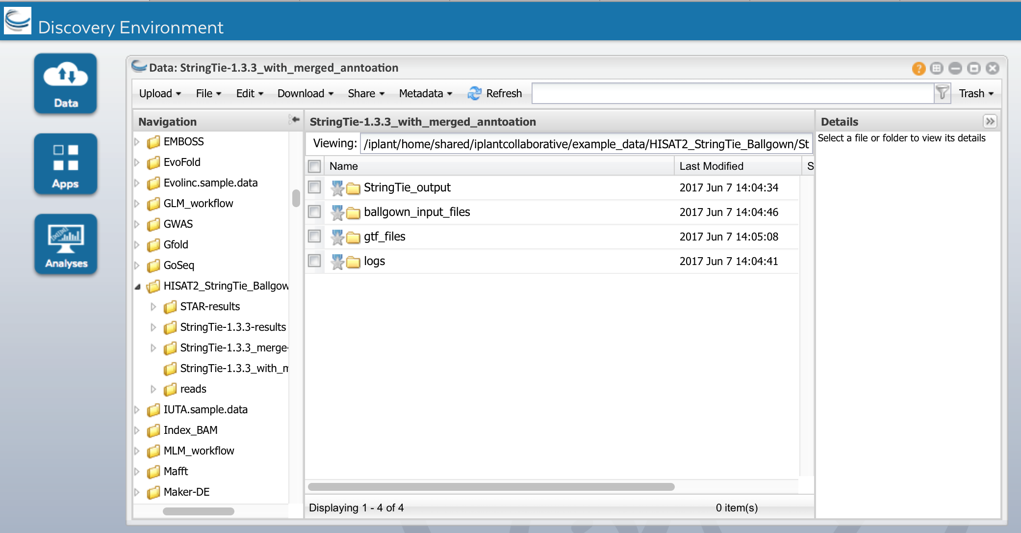
Ballgown_input_files: count files (*ctab files) for each sample
e_data.ctab: exon-level expression measurements.
i_data.ctab: intron- (i.e., junction-) level expression measurements
t_data.ctab: transcript-level expression measurements
e2t.ctab: table with two columns, e_id and t_id, denoting which exons belong to which transcripts
i2t.ctab: table with two columns, i_id and t_id, denoting which introns belong to which transcripts
More details of the ctab files please refere the Ballgown documentation
Section 5: Compare expression analysis using Ballgown
Ballgown is a R package that uses abundance data produced by StringTie to perform differential expression analysis at gene, transcript, exon or junction level. It does both time series and fixed condition differential expression analysis.
a) In Apps select Ballgown
b) provide a experiment design matrix file in txt, This file defines samples, group and replicate information e:g
ID condition reps
IS20351_DS_1_1 DS 1
IS20351_DS_1_2 DS 2
IS20351_DS_1_3 DS 3
IS20351_WW_1_1 WW 1
IS20351_WW_1_2 WW 2
IS20351_WW_1_3 WW 3
Here we are doing a pairwise comparison for differential expression in sensitive genotype under Drought Stress(DS) and Well Watered(WW) condition. We have 3 replicates under each condition.
c) Upload the following files
- design matrix file
Community Data -> iplantcollaborative -> example_data -> HISAT2_StringTie_Ballgown -> design_matrix
- Ballgown_input_files directoey containing the ctab count files from stringtie runs
Community Data -> iplantcollaborative -> example_data -> HISAT2_StringTie_Ballgown -> StringTie-1.3.3_from_merged_annotation -> ballgown_input_files
- provide experimental covariate which is condition(it should match column in design matrix file)

d) Launch analysis
e) Examine results

Successful execution of the Ballgown will create a directory named output. The directory will contain the following files:
- Rplots.pdf- Boxplot of FPKM distribution of each smaple
- results_gene.tsv- Gene level Differential expression with no filtering
- results_gene_filter.sig.tsv- Identify genes with p value < 0.05
- results_gene_filter.tsv- Filter low-abundance genes, here we remove all genes with a variance across samples less than one
- results_trans.tsv-transcript level Differential expression with no filtering
- results_trans_filter.sig.tsv- Identify transcripts with p value < 0.05
- results_trans_filter.tsv-Filter low-abundance genes, here we remove all transcript with a variance across samples less than one
Running Ballgown for Differential gene expression and visualization in Atmosphere.
Section 1: Connect to an instance of an Atmosphere Image and launch a instance
1. Go to https://atmo.cyverse.org/ and log in with IPLANT TEST USER CREDENTIALS.

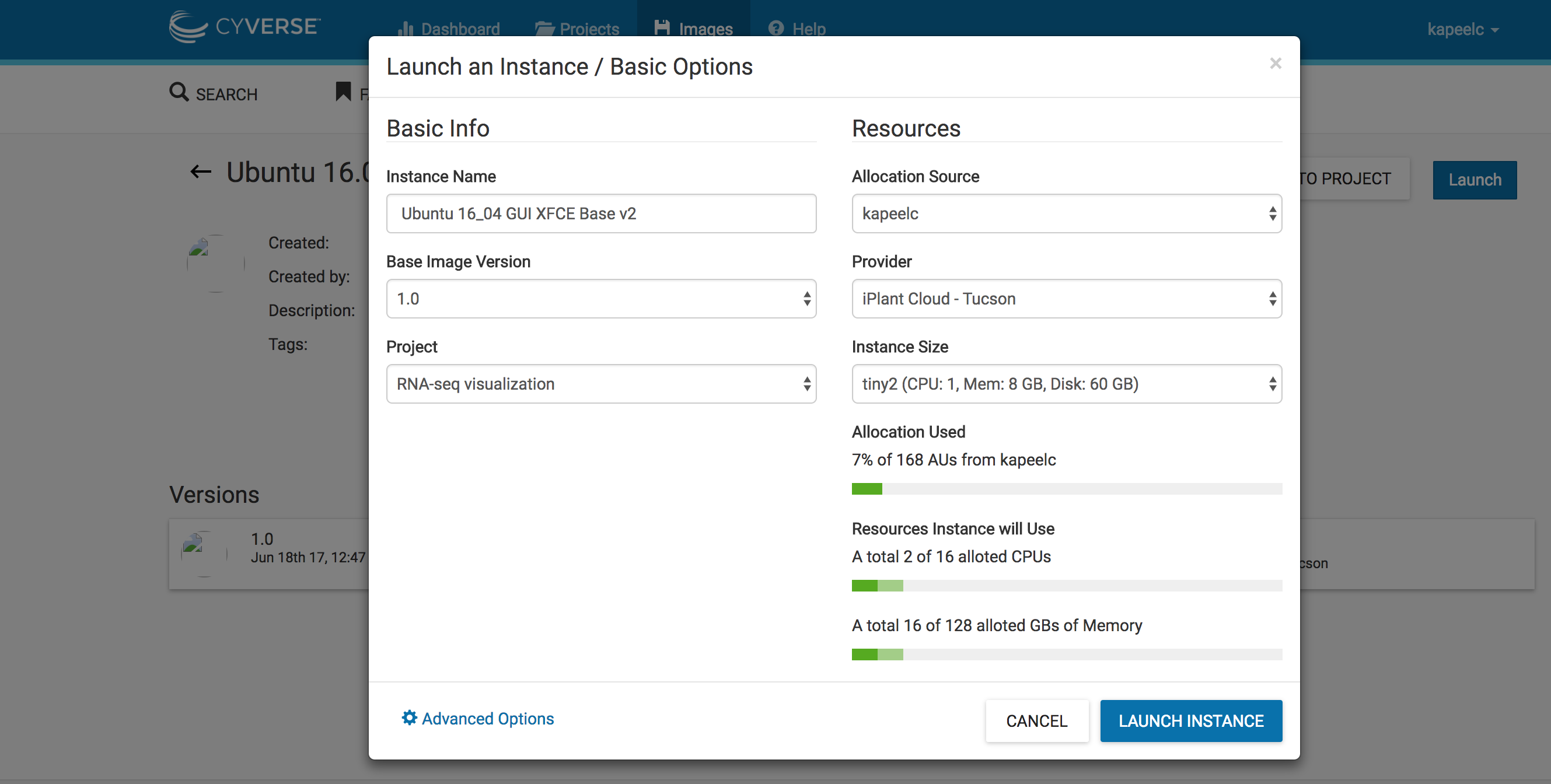
2. Click on images. Search "Ubuntu 16_04 GUI XFCE Base v2" on the search space. Click on "Ubuntu 16_04 GUI XFCE Base v2" image.

3. Click on Launch. Add to existing projects if you have already created one. In this case, we will add the instance to existing project "RNA-seq visualization". Select the size of the instance "tiny 2(CPU:1,Mem: 8, Disk: 60Gb)". Click on Launch instance. This will launch a instance of the image.
4. Once the instance is active, you will get a email confirmation and can also see the status active on the Atmosphere portal

5. Copy the IP address "128.196.64.168", if you are using MAC or Ubuntu open a terminal window and paste the IP address on the command line using your Cyverse user name and hit enter. This will ask you your Cyverse user account passowrd, hit enter
Note- After entering the password if its ask you to add your IP address to the config, enter yes.
escudilla:~ kchougul$ ssh kapeelc@128.196.64.168
After you enter the password you should see something like this
escudilla:~ kchougul$ ssh kapeelc@128.196.64.168
kapeelc@128.196.64.168's password:
Welcome to Ubuntu 16.04.2 LTS (GNU/Linux 4.4.0-72-generic x86_64)

  Get cloud support with Ubuntu Advantage Cloud Guest:
    http://www.ubuntu.com/business/services/cloud

45 packages can be updated.
0 updates are security updates.


*** System restart required ***
Welcome to
    _   _                             _
   / \ | |_ _ __ ___   ___  ___ _ __ | |__   ___ _ __ ___
  / _ \| __| '_ ` _ \ / _ \/ __| '_ \| '_ \ / _ \ '__/ _ \
 / ___ \ |_| | | | | | (_) \__ \ |_) | | | |  __/ | |  __/
/_/   \_\__|_| |_| |_|\___/|___/ .__/|_| |_|\___|_|  \___|
                               |_|
Last login: Mon Jun 19 14:16:47 2017 from 143.48.50.204
**************************************************************************
# A new feature in cloud-init identified possible datasources for        #
# this system as:                                                        #
#   ['OpenStack', 'None']                                                #
# However, the datasource used was: CloudStack                           #
#                                                                        #
# In the future, cloud-init will only attempt to use datasources that    #
# are identified or specifically configured.                             #
# For more information see                                               #
#   https://bugs.launchpad.net/bugs/1669675                              #
#                                                                        #
# If you are seeing this message, please file a bug against              #
# cloud-init at                                                          #
#    https://bugs.launchpad.net/cloud-init/+filebug?field.tags=dsid      #
# Make sure to include the cloud provider your instance is               #
# running on.                                                            #
#                                                                        #
# After you have filed a bug, you can disable this warning by launching  #
# your instance with the cloud-config below, or putting that content     #
# into /etc/cloud/cloud.cfg.d/99-warnings.cfg                            #
#                                                                        #
# #cloud-config                                                          #
# warnings:                                                              #
#   dsid_missing_source: off                                             #
**************************************************************************

Disable the warnings above by:
  touch /home/kapeelc/.cloud-warnings.skipy
or
  touch /var/lib/cloud/instance/warnings/.skip
kapeelc@vm64-168:~$
6. Now your instance is ready to use. We first download the data (Section 4 "/iplant/home/shared/iplantcollaborative/example_data/HISAT2-StringTie-Ballgown/StringTie-1.3.3_from_merged_annotation/ballgown_input_files") needed to run Ballgown. We create a directory ballgown_analysis to download the input files. We will use Rstudio on atmosphere to do the interactive analysis using Ballgown R package. To download the data we will use command line icommands that are installed in this instance for you. Type the below command on the terminal where the instance is opened and enter your cyverse password to begin download
1. kapeelc@vm64-135:~$ mkdir ballgown_analysis
2. kapeelc@vm64-168:~$ iget -PVr /iplant/home/shared/iplantcollaborative/example_data/HISAT2-StringTie-Ballgown/StringTie-1.3.3_from_merged_annotation/ballgown_input_files
NOTICE: created irodsHome=/iplant/home/kapeelc
NOTICE: created irodsCwd=/iplant/home/kapeelc
NOTICE: created irodsHome=/iplant/home/kapeelc
NOTICE: created irodsCwd=/iplant/home/kapeelc
NOTICE: created irodsHome=/iplant/home/kapeelc
NOTICE: created irodsCwd=/iplant/home/kapeelc
NOTICE: created irodsHome=/iplant/home/kapeelc
NOTICE: created irodsCwd=/iplant/home/kapeelc
NOTICE: created irodsHome=/iplant/home/kapeelc
NOTICE: created irodsCwd=/iplant/home/kapeelc
NOTICE: created irodsHome=/iplant/home/kapeelc
NOTICE: created irodsCwd=/iplant/home/kapeelc
NOTICE: created irodsHome=/iplant/home/kapeelc
NOTICE: created irodsCwd=/iplant/home/kapeelc
Enter your current iRODS password:

3. kapeelc@vm64-135:~$ iget -PV /iplant/home/shared/iplantcollaborative/example_data/HISAT2-StringTie-Ballgown/design_matrix .
Once the down load is complete you should see the directory which contains the ctab count files for each sample that will be used in Ballgown for differential expression and plotting
kapeelc@vm64-168:~$ ls -lh
total 36K
drwxr-xr-x 3 kapeelc iplant-everyone 4.0K Jul  19 13:50 ballgown_analysis
drwxr-xr-x 2 root root 4.0K Jun 19 13:50 Desktop
drwxr-xr-x 2 kapeelc iplant-everyone 4.0K Jun 19 13:50 Documents
drwxr-xr-x 2 kapeelc iplant-everyone 4.0K Jun 19 13:50 Downloads
drwxr-xr-x 2 kapeelc iplant-everyone 4.0K Jun 19 13:50 Music
drwxr-xr-x 2 kapeelc iplant-everyone 4.0K Jun 19 13:50 Pictures
drwxr-xr-x 2 kapeelc iplant-everyone 4.0K Jun 19 13:50 Public
drwxr-xr-x 2 kapeelc iplant-everyone 4.0K Jun 19 13:50 Templates
drwxr-xr-x 2 kapeelc iplant-everyone 4.0K Jun 19 13:50 Videos
Section 2: Using R studio on atmosphere to do the interactive analysis using Ballgown R package
- On the command line type below three commands to start a Rstudio and enter your Cyverse password. This will install all the dependencies needed to start Rstudio.
1. kapeelc@vm64-135:~$ sudo apt-get update && sudo apt-get -y install gdebi-core r-base libxml2-dev
[sudo] password for kapeelc:
2. kapeelc@vm64-135:~$ wget https://download2.rstudio.org/rstudio-server-1.0.136-amd64.deb
3. kapeelc@vm64-135:~$ sudo gdebi -n rstudio-server-1.0.136-amd64.deb
2. If you want to find what the IP address of the R studio then run below command,
kapeelc@vm64-135:~$ echo My RStudio Web server is running at: http://$(hostname):8787/
My RStudio Web server is running at: http://vm64-135.iplantcollaborative.org:8787/
just copy and paste http://vm64-135.iplantcollaborative.org:8787/ on to the web-browser
3. Enter your Cyverse user name and password to launch the R studio on browser

4. paste the below R commands to begin the analysis. Start File -> New File -> R script, then paste the commands
